Precision, Accuracy, and Error Analysis in Measurements

When performing experiments or collecting data, it’s important to not only take measurements but also understand how reliable and valid those measurements are. Concepts like precision, accuracy, and error propagation are fundamental in engineering and science.

Precision v Accuracy

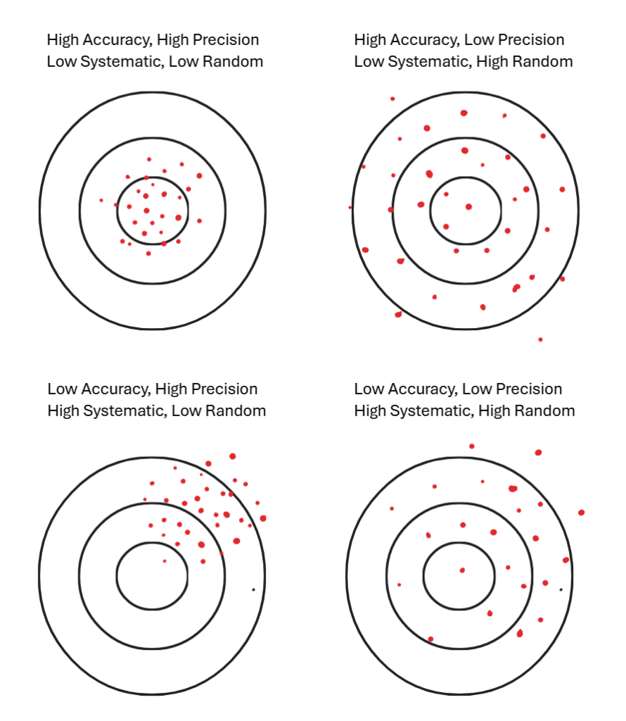
Precision is the spread of results or the reproducibility of the data. A high precision would mean a low standard deviation and a low precision would mean a large standard deviation.

Accuracy is how close a measurement is to the “true” value. This would be how close your data points or your sample mean is to the true mean.

Random v Systematic Errors

Random errors will vary the data unpredictably from one measurement to another and affect precision. Systematic error will result in a consistent skew of your data in one direction and this will affect accuracy.

You often see this represented by four target diagrams:

High accuracy + high precision (tight cluster at bullseye)
High precision but low accuracy (tight cluster off-center)
High accuracy but low precision (spread out but centered on bullseye)
Low accuracy and low precision (spread out and off-center)

However, in practice we don’t have “targets,” so distinguishing them can be very difficult.

Random Error v Systematic Error Quantitative

For a random error:

P(+ , \text{error}) = P(- , \text{error})

This means that the probability of having a data point above the mean or below the mean is the same. Over many trials (large N), the random errors cancel each other out, and the sample mean approaches the true mean.

We can estimate:

% , \text{error} = \frac{1}{\sqrt{N}}

For systematic errors:

P(+ , \text{error}) \neq P(- , \text{error})

This means that even for large N, your sample mean will remain offset.

How to Detect Systematic Errors

Analyze blank samples or samples of known composition. This will give us a reference point that we can now calibrate to.
Compare results with different measurement techniques. If we use two different experimental methods, we can compare the accuracy of the two and determine if there are any systematic errors with one of the techniques.
Recalibrate instruments frequently.

Propagation of Error

When combining measurements that each have their own uncertainties, we must calculate how those errors combine.

Sums and Differences

The upper bound of uncertainty is given by the sum of the uncertainties.

If we measure $x$ and $y$ with uncertainties $e_x$ and $e_y$ :

e_{tot} = e_x + e_y

For subtraction:

(x - y) \pm e_{tot}

Products and Quotients

For multiplication or division, the fractional (percentage) uncertainties are added:

\frac{e_y}{y} = \frac{e_{x1}}{x_1} + \frac{e_{x2}}{x_2} + \frac{e_{x3}}{x_3} + \dots

Example:

If $y = \frac{x_1 x_2}{x_3}$ , then

%e_y = %e_{x1} + %e_{x2} + %e_{x3}

Multiplying by a constant does not change the fractional uncertainty.

Powers and Logs

For powers:

If $y = x^a$ , then

\frac{e_y}{|y|} = |a| \frac{e_x}{|x|}

or equivalently:

%e_y = |a| \cdot %e_x

Example:
If $y = x^2$ and $%e_x = 3%$ , then

%e_y = 2 \cdot 3% = 6%

For logarithms:

If $y = \log_x z$ ,

e_y = \frac{1}{z \ln(x)} e_z

Example:
If $y = \ln(z)$ and $z = 10 \pm 0.5$ , then

e_y = \frac{1}{10} (0.5) = 0.05

So $y = \ln(10) \pm 0.05$ .

Independence in Uncertainty

If errors are uncorrelated (true random fluctuations), then adding them linearly overestimates the uncertainty. Instead, use the sum in quadrature:

For addition/subtraction:

e_y = \sqrt{e_{x1}^2 + e_{x2}^2 + e_{x3}^2 + \dots}

For multiplication/division, apply the same rule but with percentage errors:

%e_y = \sqrt{(%e_{x1})^2 + (%e_{x2})^2 + \dots}

Use quadrature only when errors are independent and random. If errors are correlated or systematic, you must add them directly.

Propagation by Steps

In more complex formulas, break the calculation into smaller steps:

Propagate the error for each intermediate step.
Carry forward the new value and its uncertainty.
Continue until the final result.

Example:

Suppose $y = \frac{(a+b)}{c}$

First calculate $d = a+b$ with $e_d = \sqrt{e_a^2 + e_b^2}$ .
Then compute $y = d/c$ , and the percentage uncertainty:

%e_y = \sqrt{(%e_d)^2 + (%e_c)^2}

Summary

Error propagation rules let you calculate combined uncertainties.

Precision = reproducibility of data.

Accuracy = closeness to true value.

Random errors reduce precision but cancel out with large N.

Systematic errors reduce accuracy and do not cancel out.